Green’s function coupled-cluster (GFCC)

Methodology

GFCC is designed for the Green’s function calculation of molecular system at the coupled-cluster level. For a review of the GFCC method employed in this work, we refer the readers to Refs. [nooijen92_55], [nooijen93_15], [nooijen95_1681], [kowalski14_094102], [kowalski16_144101], [kowalski16_062512], [kowalski18_561], [kowalski18_4335], [kowalski18_214102].

Briefly, the matrix element of the retarded part of the analytical frequency dependent Green’s function of an \(N\)-electron system can be expressed as

(1)\[\begin{aligned} G^R_{pq}(\omega) = &&\langle \Psi | a_q^\dagger (\omega + ( H - E_0 ) - i \eta)^{-1} a_p | \Psi \rangle \end{aligned}\]

where \(H\) is the electronic Hamiltonian of the \(N\)-electron system, \(| \Psi \rangle\) is the normalized ground-state wave function of the system, \(E_0\) is the ground state energy, and the \(a_p\) (\(a_p^\dagger\)) operator is the annihilation (creation) operator for electrons in the \(p\)-th spin-orbital. Besides, \(\omega\) is the frequency, \(\eta\) is the broadening factor, and \(p,q,r,s,\ldots\) refers to general spin-orbital indices (we also use \(i,j,k,l,\ldots\) to label occupied spin-orbital indices, and \(a,b,c,d,\ldots\) to label virtual spin-orbital indices). By introducing bi-orthogonal CC formalism, the CC Green’s function can then be expressed as

(2)\[\begin{aligned} G^R_{pq}(\omega) = &&\langle\Phi|(1+\Lambda) \bar{a_q^{\dagger}} (\omega+\bar{H}_N- \text{i} \eta)^{-1} \bar{a}_p |\Phi\rangle \end{aligned}\]

where \(|\Phi\rangle\) is the reference function, and the normal product form of similarity transformed Hamiltonian \(\bar{H}_N\) is defined as \(\bar{H} - E_0\). The similarity transformed operators \(\bar{A}\) (\(A = H, a_p, a_q^{\dagger}\)) are defined as \(\bar{A} = e^{-T} A ~e^{T}\). The cluster operator \(T\) and the de-excitation operator \(\Lambda\) are obtained from solving the conventional CC equations. Now we can introduce an \(\omega\)-dependent IP-EOM-CC type operators \(X_p(\omega)\) mapping the \(N\)-electron Hilbert space onto an (\(N\)\(-\)1)-electron Hilbert space

(3)\[\begin{split}\begin{aligned} X_p(\omega) &=& X_{p,1}(\omega)+X_{p,2}(\omega) + \ldots \notag \\ &=& \sum_{i} x^i(p, \omega) a_i + \sum_{i<j,a} x^{ij}_a(p, \omega) a_a^{\dagger} a_j a_i +\ldots \end{aligned}\end{split}\]

that satisfies

(4)\[\begin{aligned} (\omega+\bar{H}_N - \text{i} \eta )X_p(\omega)|\Phi\rangle = \bar{a}_p |\Phi\rangle \end{aligned}\]

Substituting this expression into Eq. (2), we end up with a compact expression for the matrix element of the retarded CC Green’s function

(5)\[\begin{aligned} G^R_{pq}(\omega) = \langle\Phi|(1+\Lambda) \bar{a_q^{\dagger}} X_p(\omega) |\Phi\rangle, \end{aligned}\]

which becomes

(6)\[\begin{aligned} G_{pq}(\omega) &=& \langle\Phi|(1+\Lambda_1+\Lambda_2) \bar{a_q^{\dagger}} (X_{p,1}(\omega)+X_{p,2}(\omega)) |\Phi\rangle \end{aligned}\]

in the GFCCSD approximation (GFCC with singles and doubles) with \(X_{p,1}\)/\(\Lambda_1\) and \(X_{p,2}\)/\(\Lambda_2\) being one- and two-body component of \(X_{p}\)/\(\Lambda\) operators, respectively. The spectral function is then given by the trace of the imaginary part of the retarded GFCCSD matrix,

(7)\[A(\omega) = - \frac {1} {\pi} \text{Tr} \left[ \Im\left({\bf G}^{\text{R}}(\omega) \right) \right] = - \frac {1} {\pi} \sum_{p} \Im\left(G_{pp}^{\text{R}}(\omega) \right)~.\]

As discusseded in our previous work on this subject [kowalski14_094102], [kowalski16_144101], [kowalski16_062512], [kowalski18_561], [kowalski18_4335], [kowalski18_214102], the practical calculation of GFCCSD matrix employing the above method involves the solution of the conventional CCSD calculations (to get converged \(T\) and \(\Lambda\) cluster amplitudes), solving linear systems of the form of Eq. (4) for all the orbitals (\(p\)‘s) and frequencies of interest (\(\omega\)‘s), and performing Eq. (5). The key step is to solve Eq. (4) for \(X_p(\omega)\) for given orbital \(p\) and frequency \(\omega\), and the overall computational cost approximately scales as \(\mathcal{O}(N_{\omega}N^6)\) with the \(N_{\omega}\) being the number of frequencies in the designated frequency regime. Therefore, if a finer or broader frequency range needs to be computed, \(N_{\omega}\) would constitute a sizable pre-factor.

In the context of high performance computing, one can divide the full computational task posed by the GFCC method into several smaller tasks according to the number of orbitals and frequencies desired. In so doing, one can distribute these smaller tasks over the available processors to execute them concurrently. In this way, the overall computational cost remains the same, but the time-to-solution can be significantly reduced. In order to reduce the formal computational cost of the GFCC method, we further introduce model-order-reduction (MOR) technique in the context of the GFCC method [peng19_3185].

We can first represent Eqs. (4) and (5) as a linear multiple-input multiple-output (MIMO) system \(\mathbf{\Theta}\),

(8)\[\begin{split}\begin{aligned} \mathbf{\Theta}(\omega) = \left\{ \begin{array}{ccl} (\omega - \text{i} \eta + \bar{\textbf{H}}_N) \textbf{X}(\omega) & = & \textbf{b}, \\ \mathbf{G}^{\text{R}}(\omega) & = & \textbf{c}^{\text{T}} \textbf{X}(\omega). \end{array}\right. \end{aligned}\end{split}\]

Here, the dimension of \(\bar{\textbf{H}}_N\) is \(D\) (For the GFCCSD method, \(D\) scales as \(\mathcal{O}\)(\(N_o^2N_v\)) with \(N_o\) being the total number of occupied spin-orbitals and \(N_v\) being the total number of virtual spin-orbitals). The columns of \(\textbf{b}\) corresponding to free terms, and the columns of \(\textbf{c}\) corresponding to \(\langle \Phi | (1+\Lambda) \bar{a^\dagger_q}\). The transfer function of the linear system \(\mathbf{\Theta}\),

(9)\[\begin{aligned} \mathbf{\gamma}(\omega) = \mathbf{c}^{\mathrm{T}} \left(\omega - \text{i} \eta + \bar{\textbf{H}}_N \right)^{-1} \mathbf{b}\end{aligned}\]

describes the relation between the input and output of \(\mathbf{\Theta}\), and is equal to its output \(\mathbf{G}^{\mathrm{R}}(\omega)\) for Eq. (8).

To apply the interpolation based MOR technique for \(\mathbf{\Theta}\), we need to construct an orthonormal subspace \(\textbf{S} = \{ \textbf{v}_1, \textbf{v}_2, \cdots, \textbf{v}_m\}\) with \(m \ll D\) and \(\langle \textbf{v}_i | \textbf{v}_j \rangle = \delta_{ij}\), such that the original linear system (Eq. (8)) can be projected into to form a model system \(\hat{\mathbf{\Theta}}\),

(10)\[\begin{split}\begin{aligned} \hat{\mathbf{\Theta}}(\omega) = \left\{ \begin{array}{ccl} (\omega - \text{i} \eta + \hat{\bar{\textbf{H}}}_N) \hat{\textbf{X}}(\omega) & = & \hat{\textbf{b}}, \\ \hat{\mathbf{G}}^{\text{R}}(\omega) & = & \hat{\mathbf{c}}^{\text{T}} \hat{\textbf{X}}(\omega), \end{array}\right. \end{aligned}\end{split}\]

where \(\hat{\bar{\textbf{H}}}_N = \textbf{S}^{\text{T}} \bar{\textbf{H}}_N \textbf{S}\), \(\hat{\textbf{X}}(\omega) = \textbf{S}^{\text{T}} \textbf{X}(\omega)\), \(\hat{\textbf{b}} = \textbf{S}^{\text{T}} \textbf{b}\), and \(\hat{\mathbf{c}}^{\text{T}} = \mathbf{c}^{\text{T}} \textbf{S}\). With the proper construction of the subspace \(\textbf{S}\), we expect \(\hat{\mathbf{\Theta}}(\omega) \approx \mathbf{\Theta}(\omega)\) for designated frequency regime.

In practice, the subspace \(\textbf{S}\) is composed of the orthonormalized auxiliary vectors, \(\textbf{X}_p\), converged at selected frequencies \(\omega_k\) in a given frequency regime, [\(\omega_\text{min}\), \(\omega_\text{max}\)]. Hence, the transfer function of the reduced model \(\hat{\mathbf{\Theta}}\) interpolates the original model \(\mathbf{\Theta}\) at these selected frequencies, i.e.,

(11)\[\hat{\mathbf{G}}^\mathrm{R}(\omega_k) = \mathbf{G}^\mathrm{R}(\omega_k)\]

for \(k = 1,\ldots,m\). The sampling of the selected frequencies in the regime follows the adaptive refinement strategy described in Ref. [vanbeeumen17_4950].

Basically, one can start with a uniformly sampled frequencies in the regime to construct a preliminary level reduced order model. Then, based on the error estimates of the computed spectral function between adjacent frequencies over the entire regime, one can decide whether the corresponding midpoints between these adjacent frequencies need to be added to refine the sampling. This refinement process continues until the maximal error estimate of the computed spectral function at the entire frequency window is below the threshold or when the refined model order exceeds a prescribed upper bound.

Key Features

The Cholesky vectors are used in all the post Hartree-Fock calculations supported by the library (to save the memory cost from using the two-electron integrals). As we have shown earlier the accuracy of using Cholesky vectors in the post Hartree-Fock calculation can be well-controlled by a pre-defined Cholesky threshold [kowalski17_4179].
The GFCCSD calculation, the \(\Lambda\) in Eq. (5) is approximated by \(T^\dagger\) amplitude. Our recent tests show that this approximation gives very close results to the conventional GFCCSD results (only the positions of satellites slightly shift) but saves almost one third of the entire computational cost of CCSD/GFCCSD [peng19_3185].
The MOR technique is automatically enabled in the GFCCSD calculation, from which for a given frequency range one can either interpolate or extrapolate the GFCCSD results to obtain good approximations for the same or extended frequency range [peng19_3185].
The GFCCSD calculations are only performed for the retarded part in occupied molecular orbital space. For molecular systems, this is a good approximation, since energy gap between the occupied and virtual molecular orbital is relatively large, the contribution of the virtual molecular space to the retarded part of the Green’s function is negligible.
Concurrent computation of frequency-dependent Green’s function matrix elements and spectral function in the CCSD/GFCCSD level (enabled via MPI process groups).
Supporting multidimensional real/complex hybrid tensor contractions and slicing on both CPU and GPU.
On-the-fly Cholesky decomposition for atomic-orbital based two-electron integrals.
Direct inversion of the iterative subspace (DIIS) is customized and implemented as the default complex linear solver. Later, the default linear solver has been changed from DIIS to generalized minimal residual method (GMRES).
Gram-Schmidt orthogonalization for multidimensional complex tensors,
Model-order-reduction (MOR) procedure for complex linear systems,
Automatic resource throttling for various inexpensive operations,
Checkpointing (or restarting) calculation employing parallel I/O operations for reading (writing) tensors from (to) disk.

Example

In the following, we will use carbon monoxide as an example to demonstrate how to perform the CCSD/GFCCSD computation. Here, we want to compute the spectral function of CO molecule over [-0.50, -0.30] a.u. (i.e. [-13.60,-8.16] eV ) in the CCSD/cc-pVDZ level, and extrapolate the GFCCSD results to [-2.00,0.00] a.u. (i.e. [-54.42, 0.00] eV).

Input File

The following shows the input file for the CCSD/GFCCSD calculation.

  "geometry": {
    "coordinates": [
      "C   0.00000000     0.00000000    0.00000000",
      "O   0.00000000     0.00000000    1.128"
    ],
    "units": "angstrom"
  },
  "basis": {
    "basisset": "cc-pvdz"
  },
  "common": {
    "maxiter": 50
  },
  "SCF": {
    "tol_lindep": 1e-06,
    "conve": 1e-12,
    "convd": 1e-11,
    "diis_hist": 10
  },
  "CD": {
    "diagtol": 1e-08
  },
  "CC": {
    "threshold": 1e-06,
    "writet": true,
    "GFCCSD": {
      "gf_ip": true,
      "gf_ea": false,
      "gf_os": false,
      "gf_cs": false,
      "gf_ngmres": 10,
      "gf_maxiter": 100,
      "gf_damping_factor": 1.0,
      "gf_eta": 0.01,
      "gf_threshold": 0.01,
      "gf_omega_min_ip": -0.4,
      "gf_omega_max_ip": -0.2,
      "gf_omega_min_ip_e": -2.0,
      "gf_omega_max_ip_e": 0.0,
      "gf_omega_delta": 0.01,
      "gf_omega_delta_e": 0.01,
      "gf_omega_min_ea": 0.0,
      "gf_omega_max_ea": 0.1,
      "gf_omega_min_ea_e": 0.0,
      "gf_omega_max_ea_e": 0.1
    }
  },
  "TASK": {
    "gfccsd": true
  }

The GFCCSD section lists the options (labeled with the gf_ prefix) used in the Cholesky-based GFCCSD calculations.

gf_ngmres

| Type: Integer | Default: 10 |

The micro steps in the GMRES procedure in the GFCC calculations.

gf_maxiter

| Type: Integer | Default: 500 |

The maximum number of iterations used to solve the GFCCSD linear equation.

gf_eta

| Type: Double | Default: -0.01 |

The broadening factor \(\eta\).

gf_threshold

| Type: Double | Default: 1e-2 |

Specifies the threshold used to determine whether the GFCCSD linear equation is converged or not.

gf_preconditioning

| Type: bool | Default: true |

Toggle preconditioner.

gf_omega_min_ip

| Type: Double | Default: -0.4 |

gf_omega_max_ip

| Type: Double | Default: -0.2 |

The lower and upper bounds of a user-defined frequency range to perform interpolation.

gf_omega_min_ip_e

| Type: Double | Default: -2.0 |

gf_omega_max_ip_e

| Type: Double | Default: 0.0 |

The lower and upper bounds of a user-defined frequency range to perform extrapolation based on the interpolated model.

gf_omega_delta

| Type: Double | Default: 0.01 |

gf_omega_delta_e

| Type: Double | Default: 0.002 |

The frequency intervals used in the above two frequency ranges.

gf_nprocs_poi

| Type: Integer | Default: 0 (all) |

Number of mpi processes to use to process a single orbital.

gf_lshift

| Type: Double | Default: 1.0 |

Level shift.

gf_restart

| Type: bool | Default: false |

Enable restart for all steps of the GFCC calculation.

gf_profile

| Type: bool | Default: false |

Prints profiling information.

Output File

The following is the abstract format of the output file, where detailed information has been skipped due to the space.

...

 Hartree-Fock iterations
...

** Hartree-Fock energy = -112.7493113372152
writing orbitals to file... done.

...

Begin Cholesky Decomposition ...

#AOs, #electrons = 28 , 7

Number of cholesky vectors = 272

...

 CCSD iterations

...

Iterations converged
 CCSD correlation energy / hartree =        -0.298038798762180
 CCSD total energy / hartree       =      -113.047350135977382

...

#occupied, #virtual = 14, 42

-------------------------
GF-CCSD (omega = -0.5)
-------------------------

-------------------------
GF-CCSD (omega = -0.3)
-------------------------

spectral function (omega_npts = 21):

...

omegas processed in level 1 = [-0.5,-0.3,]

-------------------------
GF-CCSD (omega = -0.4)
-------------------------

spectral function (omega_npts = 21):

...

omegas processed in level 2 = [-0.4,]

--------extrapolate & converge--------

...

As we can see, the output file includes three major parts, namely Hartree-Fock (SCF), CCSD, and GFCCSD. The major information that can be obtained directly includes SCF energy, CCSD ground state correlation energy, GFCCSD spectral function. Since MOR technique is used by default in the GFCCSD calculation, the spectral function computed is printed out at each level. At the end of the output, the intrapolated and extrapolated spectral function over extended frequency range is also printed out.

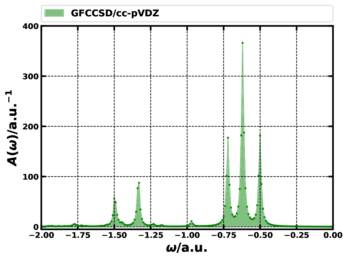
Spectral functions of the carbon monoxide molecule in the frequency regime of [-2.00, 0.00] a.u. computed by GFCCSD method employing MOR technique. \({\eta}\) = 0.01 a.u. and \(\delta\omega \le\)0.002 a.u.

Performance

At present, the GFCC has been tested for systems consisting of 100\(\sim\)1200 basis functions. For a given frequency point, the computational cost of performing GFCCSD calculation for entire molecular orbital space is \(\mathcal{O}(N^6)\), where \(N\) represents the number of basis functions. Figure below shows the running time of the GFCCSD/cc-pVDZ calculation of C\(_{60}\) molecule (\(N=840\) basis functions) at \(\omega=-10.45\) a.u. on OLCF Summit supercomputer.

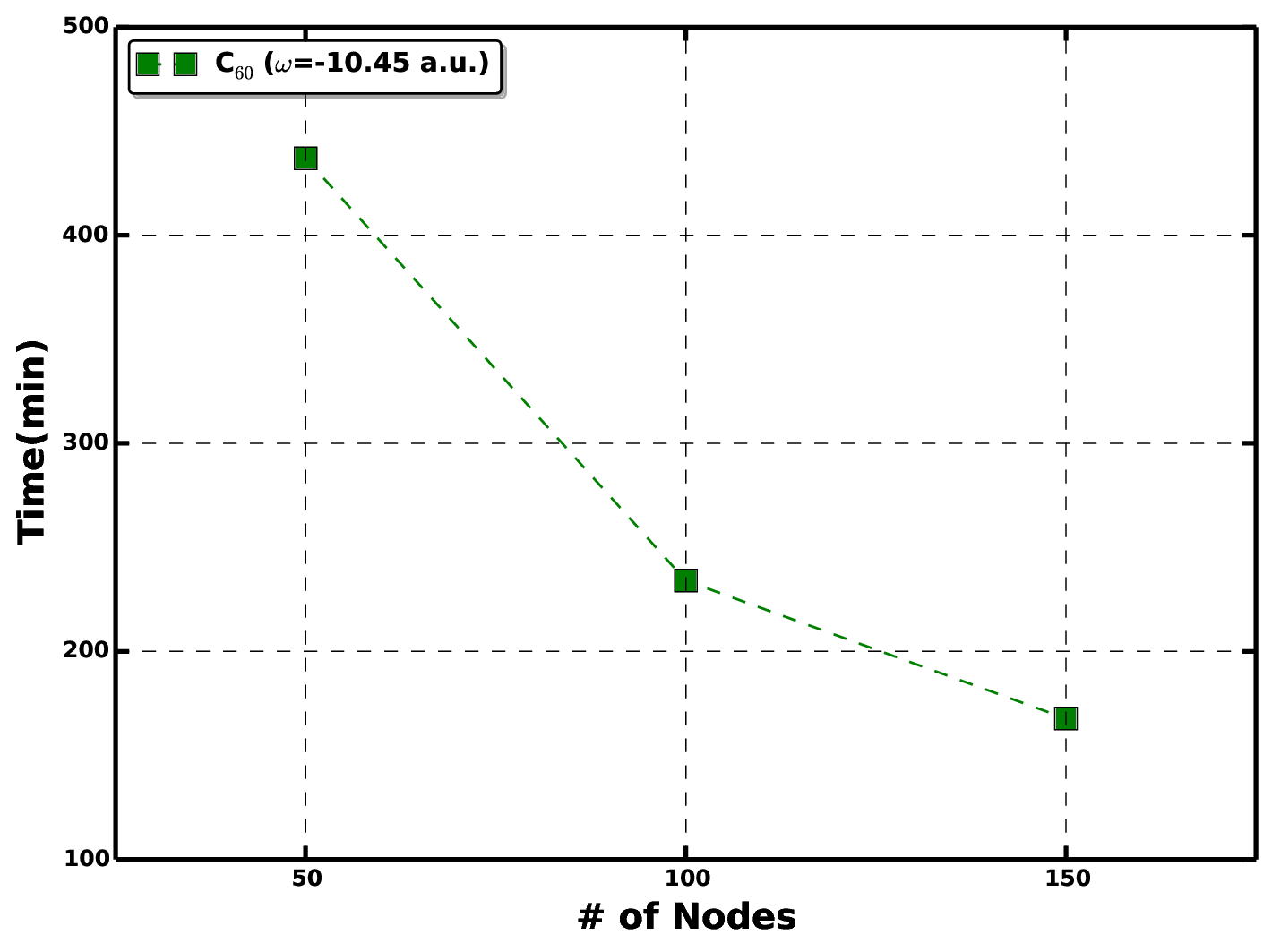
Running time as a function of number of nodes for carrying out GFCCSD/cc-pVDZ calculation of C\(_{60}\) molecule at \(\omega=-10.45\) a.u.

Citing this work

If you are referencing this GFCC implementation in a publication, please cite the following papers:

Bo Peng, Ajay Panyala, Karol Kowalski and Sriram Krishnamoorthy, GFCCLib: Scalable and Efficient Coupled-Cluster Green’s Function Library for Accurately Tackling Many Body Electronic Structure Problems, Computer Physics Communications (April 2021) DOI:10.1016/j.cpc.2021.108000.
Bo Peng, Karol Kowalski, Ajay Panyala and Sriram Krishnamoorthy, Green’s function coupled cluster simulation of the near-valence ionizations of DNA-fragments, The Journal of Chemical Physics 152, 011101 (Jan 2020) DOI:10.1063/1.5138658.

Acknowledgments

The development of GFCC is supported by the Center for Scalable, Predictive methods for Excitation and Correlated phenomena (SPEC), which is funded by the U.S. Department of Energy (DOE), Office of Science, Office of Basic Energy Sciences, the Division of Chemical Sciences, Geosciences, and Biosciences.